CBE 255. Introduction to Chemical Process Modeling

CBE Faculty

Department of Chemical and Biological Engineering

University of Wisconsin

Madison, Wisconsin

Course Overview

This course provides an overview of the chemical engineering curriculum and develops facility with using modern computational software for numerical problem solving.

The course provides an integrative overview of the entire chemical engineering curriculum. The faculty instructors for the latter courses in the curriculum have identified the key modeling concepts that they would like students entering their courses to be exposed to early in their education in our department. We will select 10-12 key topics from this list and structure the course around one key concept per week. The lectures will introduce these concepts and the students will immediately begin to apply them in smaller discussion sections. We will introduce computational tools motivated by these key concepts. By the end of this course, the students will have a set of tools that have been selected by the faculty in the latter courses as most useful to them as instructors.

Technology is an essential component of this course. The college has invested in classrooms with laptop projection capability and wireless internet connections. Many engineering undergraduates bring their own laptops to campus. The department will loan the additional laptops so every student can bring their laptop to class. The course requires intensive problem solving in small groups to educate the students in how to use advanced computational tools for engineering decision making in complex situations. We envision using undergraduates who have mastered the course in previous semesters as the leaders for the smaller discussion sections. The professor in charge of the course will also cover one discussion section on a rotating basis.

The course may be broken into two parts, with the first part taught to sophomores and the second part to juniors. In this way, the students will find almost immediate use of all the tools they have learned in their next semester courses.

Given the following features: (i) the course provides an integrated view of the entire curriculum, (ii) the course instructors select the concepts and computational tools presented, and (iii) the senior students lead discussion sections with the junior students, we hope to foster a learning community in the department in which using technology to solve complex engineering problems becomes an integral part of our students' educational experience.

Complete collections of the M-files for both Matlab and Octave in zip or tar.gz file formats are available for download from the following links:

Matlab:

cbe255-matlab-m-files-v1.0.zip

Octave:

cbe255-octave-m-files-v1.0.zip

Module 1: Programming and programming languages

Programming concepts: introduction to Matlab, purpose of Matlab windows, accessing the online help system.

Video Lectures

1.1 MATLAB Introduction (9 min)

1.2 Accessing MATLAB and CAE Files (6 min)

1.3 Graphing (58 min)

1.4 Linear Algebra (40 min)

1.5 Matrix Examples (21 min)

1.6 Functions (40 min)

1.7 Function Examples (23 min)

1.8 Conditions and If Statements (38 min)

1.9 If Examples (11 min)

1.10 For Loops (35 min)

1.11 Examples with For Loops (34 min)

1.12 Termination (29 min)

Module 2: Stoichiometry of chemical reactions

Chemical and biological engineering concepts: chemical reactions, linear independence of reactions, reaction rates, production rates

Computational concepts: matrices, rank of a matrix, submatrices, reshaping matrices, solving least squares problems

Programming concepts: looping, conditionals, plotting, loading data from files, writing to the screen

Broader applications of these concepts: electrical circuit theory, network models, linear programming and game theory, financial models and optimization

Tutorial 2

Video Lectures

2.1 Stoichiometry and Rates (42 min)

2.2 Estimating Reaction Rates (52min)

Module 3: Diffusion and heat transfer

Chemical and biological engineering concepts: heat transfer and mass diffusion, gradient and flux, thermal conductivity, heat capacity, diffusivity, dimensionless variables

Computational concepts: partial differential equations, implicit differential equations, differential-algebraic equations, orthogonal collocation, semi-infinite domains

Programming concepts: colloc program, functions, scripts, global statement, ODE solvers in Matlab, ode15i

Broader applications of these concepts: transport phenomena, rate processes, dimensional analysis

Tutorial 3

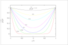
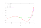
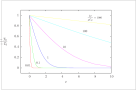
	Figure 2 (page 6): Temperature profile at several times during heating of a slab; various kt/(\rho C_Pb^2).			Figure 3 (page 7): Temperature profile of the semi-infinite slab at different \tau = kt/(\rho C_P).
	Figure 5 (page 12): Dimensionless concentration versus dimensionless radial position for different numbers of collocation points.			Figure 6 (page 13): Relative error in the effectiveness factor versus number of collocation points.
	Figure 7 (page 15): The solution to the full model for the series reaction A -> B -> C; ODE model.			Figure 8 (page 15): The solution to the reduced QSSA model; DAE model.
	Figure 9 (page 18): The function sin 2 \pi x and 10 collocation points.			Figure 10 (page 19): The function e^{-10x} and 10 collocation points.

Module 4: Process systems steady-state modeling and design

Chemical and biological engineering concepts: process systems, reaction, separation, flash tank, recycle, material balances, degrees of freedom

Computational concepts: solving sets of nonlinear algebraic equations, Newton's method, Jacobian matrix

Programming concepts: looping, iteration, formatted output to the screen, user input from the keyboard, nonlinear algebraic equation solvers in Matlab

Tutorial 4

Figure 2 (page 5):
Two iterations of Newton's method for f(x) = x^3 - 2x^2 + 3x - 6 = 0.

Video Lectures

4.1 Newtons Method (31 min)

4.2 Roots, Fzero, & Anonymous Functions (31 min)

4.3 Process System (24 min)

4.4 Fsolve (32 min)

Module 5: Chemical kinetics in well-mixed reactors

Chemical and biological engineering concepts: chemical kinetics, law of mass action, material balance, well-mixed reactor, reaction rates, production rates, complex dynamics, oscillations, Zhabotinsky reaction, coupled mass and energy balance for the CSTR

Computational concepts: ordinary differential equations, Euler method, stepsize, relative and absolute errors

Programming concepts: functions, scripts, global statement, ODE solvers in Matlab, ode15s

Broader applications of these concepts: dynamical systems, complex dynamics, oscillations, multiple steady states

Tutorial 5

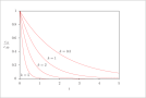
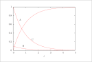
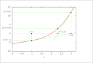
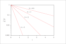
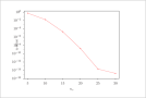
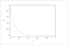
	Figure 2 (page 3): First-order, irreversible kinetics in a batch reactor.			Figure 3 (page 3): First-order, irreversible kinetics in a batch reactor, log scale.
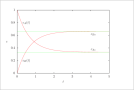
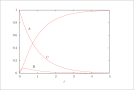
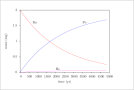
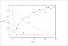
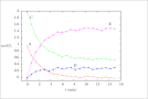
	Figure 4 (page 6): First-order, reversible kinetics in a batch reactor, k_1=1, k_{-1}=0.5, c_{A0}=1, c_{B0}=0.			Figure 5 (page 7): Concentrations of species in Reactions \ref {rxn:radio1}--\ref {rxn:radio2} versus time.
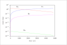
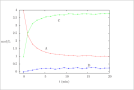
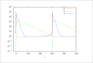
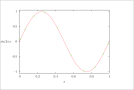
	Figure 6 (page 8): Concentrations (log scale) versus time			Figure 8 (page 16): Complex dynamic behavior of the Oregonator model of the Belousov-Zhabotinsky reaction.

Video Lectures

5.1 Eulers Method (34 min)

5.2 Single ODEs (25 min)

5.3 Reactor ODEs (36 min)

5.4 Multiple ODEs (40 min)

5.5 ode15s tspan (6 min)

Module 6: Staged separations

Tutorial 6

Module 7: Estimating parameters from data

Chemical and biological engineering concepts: fitting chemical and biological engineering models to data

Computational concepts: optimization, least squares, statistical confidence intervals, normal and uniform distributions, sampling, mean, variance

Programming concepts: parest.m, ellipse.m, Sundials package, hist, chi2inv, sqrtm, rand, randn

Broader applications of these concepts: Decision making under uncertainty, model discrimination, statistical methods, random variables, sampling

Tutorial 7

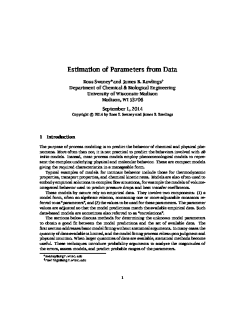
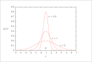
	Figure 1 (page 3): Normal distribution, with probability density p_\xi (x) = (1/\sqrt {2\pi \sigma ^2}) o{exp}(-(1/2) (x-m)^2/\sigma ^2).			Figure 2 (page 4): Multivariate normal for n=2.
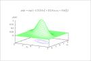
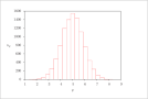
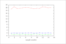
	Figure 4 (page 7): Histogram of 10,000 samples of {\sc Matlab}'s randn function.			Figure 5 (page 10): The 15 samples of measurement, pressure, and concentration.
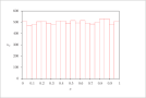
	Figure 6 (page 12): Histogram of 10,000 samples of uniformly distributed x.			Figure 7 (page 12): Histogram of 10,000 samples of y= sum_{i=1}^{10} x_i.
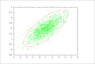
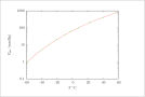
	Figure 8 (page 14): One thousand samples of the random variable x\sim N(m, P) and 95% probability contour.			Figure 10 (page 20): Antoine model fitted to the acetone vapor pressure data of Example \ref {ex:AntoineFit}.
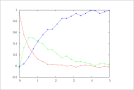
	Figure 11 (page 22): Measurements of species concentrations in Reactions \ref {rxn:series} versus time.			Figure 12 (page 23): Fit of model to measurements using estimated parameters.
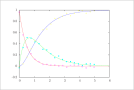
	Figure 13 (page 26): Measurements of species concentrations versus time for parallel reactions.			Figure 14 (page 31): Measurements of species concentrations versus time for Exercise\ref {exer:ABCD}.
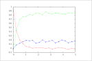
	Figure 15 (page 32): Measurements of species concentrations versus time for Exercise\ref {exer:ABCD_lowB}.			Figure 16 (page 33): Rate versus concentration of A.
	Figure 17 (page 35): Concentrations of species A, C, D, and E versus time.

Video Lectures

7.1 Parameter Estimation (32 min)

7.2 More Parameter Estimation (32 min)

7.3 ODE Parameter Estimation (45 min)

Module 8: Course review

Tutorial 8