Figure 11 (page 22):

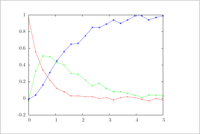
Measurements of species concentrations in Reactions \ref {rxn:series} versus time.

Code for Figure 11

Text of the GNU GPL.

main.m

clear('all'); close('all');
%
% Create data for the A->B->C model
% jbr,  11/2008

clear all
close all
global theta

k1 = 2;
k2 = 1;
ca0 = 1;
cb0 = 0;
cc0 = 0;
c0 = [ca0; cb0; cc0];
theta = [k1; k2];
tfinal = 5;
nplot = 100;



measure.states = [1,2,3];
measure.time = linspace(0, tfinal, 20)';

%create the measurements by solving the model and adding noise
[tsolver, cabc] = ode15s(@massbal, measure.time, c0);
randn('seed',0);
y  = cabc(:,measure.states);
measure.data = y + 0.02*randn(size(y));
myfile = fopen('ABC_data.dat', 'w');
for i = 1: size(y,1)
  fprintf(myfile, '%8.2f', measure.time(i), measure.data(i,:));
  fprintf(myfile, '\n');
end
fclose(myfile);

figure(1);
plot(measure.time, measure.data, '-o')

massbal.m

function xdot = massbal(t, x)
  global theta
  ca  = x(1);
  cb  = x(2);
  cc  = x(3);
  k1  = theta(1);
  k2  = theta(2);
  r1 = k1*ca;
  r2 = k2*cb;
  xdot = [-r1; r1-r2; r2];