Figure 10 (page 20):

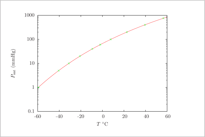
Antoine model fitted to the acetone vapor pressure data of Example \ref {ex:AntoineFit}.

Code for Figure 10

Text of the GNU GPL.

main.m

clear('all'); close('all');
% Vapor pressure values (data?) from Perry's 7th Table 2-8 p. 2-61.
% Psat [=] mmHg, T [=] degC

% The table values seem to have been smoothed, perhaps even with Antoine.
% Should add some noise...

data = [ -59.4	1 ; ...
         -40.5	5 ; ...
         -31.1	10 ; ...
         -20.8	20 ; ...
          -9.4  40 ; ...
          -2.0  60 ; ...
           7.7  100 ; ...
          22.7  200 ; ...
          39.5  400 ; ...
          56.5  760 ] ;
Psat = data(:,2);
T = data(:,1);

% Error for pressure is given as a relative error (2 %).  This is
% equivalent to an absolute error in the log of the value.  Therefore, we
% will chose to fit y = f(x,theta), taking y = ln Psat and x = T.

sigmax = 0.2;
sigmay = 0.02;  % This is an approximation, good enough in this situation.
                % (Could use log(1.02) .)
                



% Both data and Antoine function give pressure values, not logs, so
% define a function handle for ln Psat and compute log of data values

lnPsat = @(T, theta) log( Antoine(T, theta) );

y = log(Psat);

% Define a function handle for the minimization objective.
% theta is a row vector, T is a column, so make
%  X = [ theta, xhat' ]
% with theta = [ A, B, C ]

% First look carefully at how we constructed function SS.
% Then make the function handle phi so SS(...) can be called in the form phi(X):

phi = @(X) SS( lnPsat, X(1:3), y, T, X(4:end)', sigmay, sigmax) ;

% Initial estimates for xhat
xhat0 = T;

% Initial estimates for parameters A, B, C

A = 16.8
B = -2994
C = 238
theta0 = [ A; B; C ];

X0 = [ theta0; xhat0 ];
%options = optimset( 'MaxFunEvals', 1000, 'TolFun', 1.e-16, 'TolX', 1.e-6);
options = optimset( 'TolFun', 1.e-16, 'TolX', 1.e-16 );
[ X, SSmin ] = fminsearch( phi, X0, options );

% Report Antoine coefficients

theta = X(1:3);
A = theta(1)
B = theta(2)
C = theta(3)

% Report average scaled error

ase = sqrt( SSmin/(length(Psat) - 3) );
disp('Average scaled error:'), disp(ase)
disp('Predicted error in T:'), disp(ase*sigmax)
disp('Predicted relative error in Psat:'), disp(ase*sigmay)


% Plot

semilogy( T, Psat,'ob' )
ylabel('Psat, mmHg')
xlabel('T, deg C')
hold on
fplot( @(T)  Antoine(T, theta), [ -60, 60 ] )

% save results to file for plotting
Tplot = linspace(-60, 60, 100)';
Pplot = Antoine(Tplot, theta);
save acetone_data.dat data;
fit = [Tplot, Pplot];
save acetone_fit.dat fit

Antoine.m

function Psat = Antoine(T, theta)
% Computes the vapor pressure using the Antoine model
%
%  ln Psat = A + B/(T + C)
%
% theta = [ A, B, C ]

A = theta(1);
B = theta(2);
C = theta(3);

Psat = exp( A + B./(T + C) );

SS.m

function result = SS( f, theta, y, x, xhat, sigmay, sigmax)
% Sum of squares function
% yhat = f(xhat,theta).  Multiple output variables are row vectors. 
% y, x = observed values
% xhat = fitted values of x.  Multiple inputs variables are in rows.
% theta = parameters

Ny = size(y,2);
Nx = size(x,2);
K = size(y,1);

% Nested loops sum over observations, xhat's, yhat's:

result = 0.;
xhat = xhat.';
for k = [1 : K]
    yhat = f(xhat(k,:), theta);
    for i = [1 : Ny ]
        eps = (yhat(i) - y(k,i))/sigmay(i);
        result = result + eps*eps;        
    end
    for j = [1 : Nx ]
        eps = (xhat(k,j) - x(k,j))/sigmax(j);
        result = result + eps*eps;        
    end
end