Figure 6 (page 8):
Concentrations (log scale) versus time
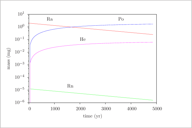
Code for Figure 6
Text of the GNU GPL.
main.m
clear('all'); close('all');
% solves the radium -> radon -> polonium
% transient decay
%
% jbr, 8/30/2007
%
global k1 k2

t1half = 1620;      % yr
t2half = 3.83/365;  % yr
samplemass = 2;     % mg
% molecular weights  g/mol
MA = 226;  % radium
MB = 222;  % radon
MC = 218;  % polonium
MD = 4;    % alpha particle

% initial conditions in moles per sample volume
nA0 = samplemass/MA;
nB0 = 0;
nC0 = 0;
nD0 = 0;
% rate constants
k1 = log(2)/t1half;
k2 = log(2)/t2half;

% times for output
time = linspace(0, 3*t1half, 100)';


x0 = [nA0; nB0; nC0; nD0];

[tout, x] = ode15s (@rates, time, x0);
% convert to mass per sample volume
% scale each column of x (species) by its mol wt
xmass = x*diag([MA, MB, MC, MD]);

figure(1);
plot(tout, xmass)
figure(2);
% clip off first time point, log(0)  undefined
semilogy(tout(2:end), xmass(2:end,:))

table = [tout, xmass];
rates.m
function rhs = rates(t, x)
  global k1 k2
  na = x(1);
  nb = x(2);
  nc = x(3);
  nd = x(4);
  r1 = k1*na;
  r2 = k2*nb;
  rhs = [-r1; r1 - r2; r2; r1 + r2];